|
Drop-down menus or drop-down lists are an easy way to elevate your Excel document. They make forms look professional and make it easy for the user to make a selection that is uniform in phrasing and formatting. This can be extremely helpful if you use the drop-down selection for a lookup to populate other data. We’ll cover how to set up a single drop-down menu, a dependent drop-down menu where the first selection triggers the options for the second menu, and a drop-down that triggers a lookup to pull in a result based on the selection. 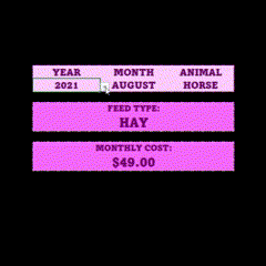 Basic Drop-Down MenuTo set up a basic drop-down menu, you need to create a list of your menu options. For my example, I have a list of animals that I would like to be the options in my drop-down. 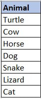 Next, we need to decide where the drop-down will live. I have created an Animal header and want the drop-down to live in the cell under that in A2. First, I will click into A2, then go to Data>Data Tools>Data Validation. If you are on a smaller screen, it may just be a small icon next to Text to Columns. 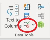 When you click the icon, you will open the Data Validation popup. You will use the drop-down menu under Allow to select List. This will change the next options to now have a Source field. You can either type in the location of your list, or you can click and select the cells that contain your list. Since my list of Animals is in K2 through K8, I have selected those cells. It automatically locked my cells with the “$” which is great because if I were to drag my data validation down so I have multiple cells with the drop-down, it will continue to pull the same list. 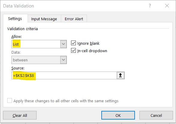 You can also name the range that contains your list and use that name in your source. Click this link to learn how to name ranges and manage them. 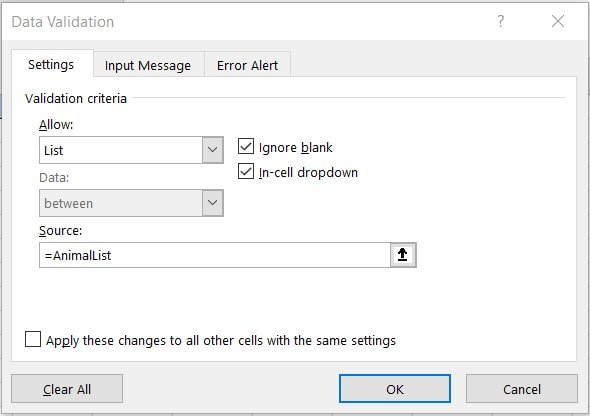 You’ll see you now have a little arrow button when you click into A2. 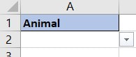 If you click that button, you will see your list appear and you can select off of the options from your list. 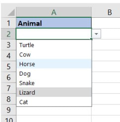 When you select from your list, your selection will display in the cell. 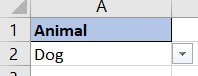 If you want to clear your selection, you can select the cell and hit delete. This will still keep your drop-down list active, but just clear your selection. To remove your drop-down completely, select the cell, go back to Data Validation as if you were going to set it up but instead click Clear All and then OK. 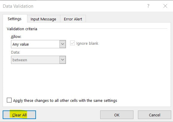 Dependent Drop-DownsIf we have multiple lists that we want to have shown in a drop-down based on what the first selection is, we can create a dependent drop-down. For our example, you will first select an animal class (mammal or reptile) and then the second list will give you the animals that belong to that class. For this, we will need to name each of our lists with the same name as the label that exists in the first drop-down. For example, if in the first list we have Mammal and Reptile, then we need to name our list of mammals as “Mammal” so when Mammal is selected, Excel is able to match the range. We will start with the first drop-down which will follow the same set up as above: Data>Data Tools>Data Validation and select List under Allow and your list range or range name under Source. Next, we need to add our drop-down for the dependent cell. We will start with the same steps Data>Data Tools>Data Validation and select List under Allow. For the Source, instead of selecting a range of cells or your named range, you are going to use the formula =INDIRECT(A2) where A2 is the cell that your primary drop-down is.  This is looking in A2 for the range name and then pulls the list for that range. 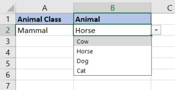 Using a Drop-Down in a DashboardIn creating dashboards, a drop-down might be a useful tool to help your user filter right to the data that they’re interested in without having to look through all of the information. For my example, I have a data set with the Feed Cost for each of my individual animals for the past two years by month. I also have the animal type, animal’s name, and the feed type. I want to create a dashboard where I can select which month, year, and animal to see what the feed type is and what the feed cost was that month. Since my data set is so long, I don’t want to create my drop-down list directly from the data since I will have so many duplicate labels. I started by creating a separate section with the headers of the drop-downs that I wanted to include and then used =UNIQUE(M3:M74) to pull a list of unique values from my data for Year. I repeated this for Month, Animal, and Feed Type. 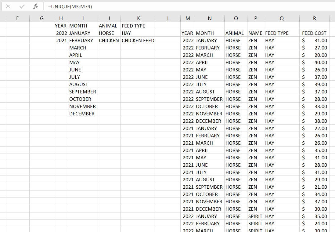 Where I want my dashboard to be built, I set up my drop-ship for each of these columns. 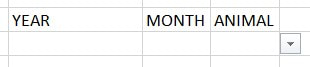 I want my dashboard to display the feed type and the feed cost, so first I will use the dropdown option for Animal to do a XLOOKUP for the feed type. If you need a refresher on XLOOKUP, check out my guide. 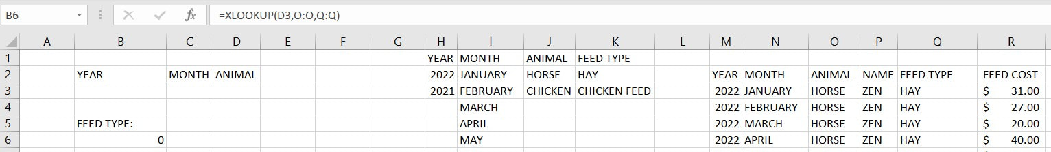 When I select an animal, the feed type now populates. Since each of my animal types only eats one type of food, this works perfectly. If I had changed my food type at a certain point in time, I would also include the year and month to pull in the feed type in that year and month. 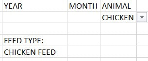 Next, I want to show the total feed cost when a year, month, and animal is selected. Since I have multiple horses, I want this to be a sum instead of a lookup so I can see my total cost for all of my horses. For this, I will use =SUMIFS since I have multiple conditions with year, month, and animal. 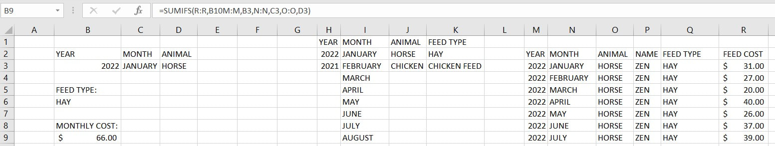 Now, if I change any of my drop-downs, my results will automatically update. 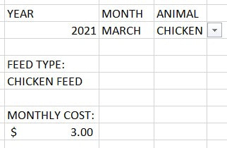 This is exactly what I wanted, but it’s just not very pretty. With some formatting, we can get this to look a little nicer. 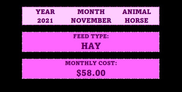 Now we have a really nice looking dashboard that we can adjust and include in our presentations. I'd love to hear what you plan on using drop-down menus for! Let me know in the comments below.
1 Comment
Nick
5/4/2023 09:47:59 am
Great in-depth explanation of drop-down menus. I will have to try them soon! Leave a Reply. |
|||
