|
We are now halfway through the year, can you believe it? At the new year, I posted a goal tracker that you could download, fill in your goals, and track your progress. This tracker included a tab dedicated to a visual chart to help you see how much progress you’ve made, which is great, but did you know you can use conditional formatting to add data bars in your cells for a quick visual of your progress without creating a chart? You can insert data bars into your cells for a quick visual. 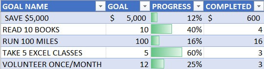 Our original tracker has a bar chart, which is also a great visual, but gives you a different result. 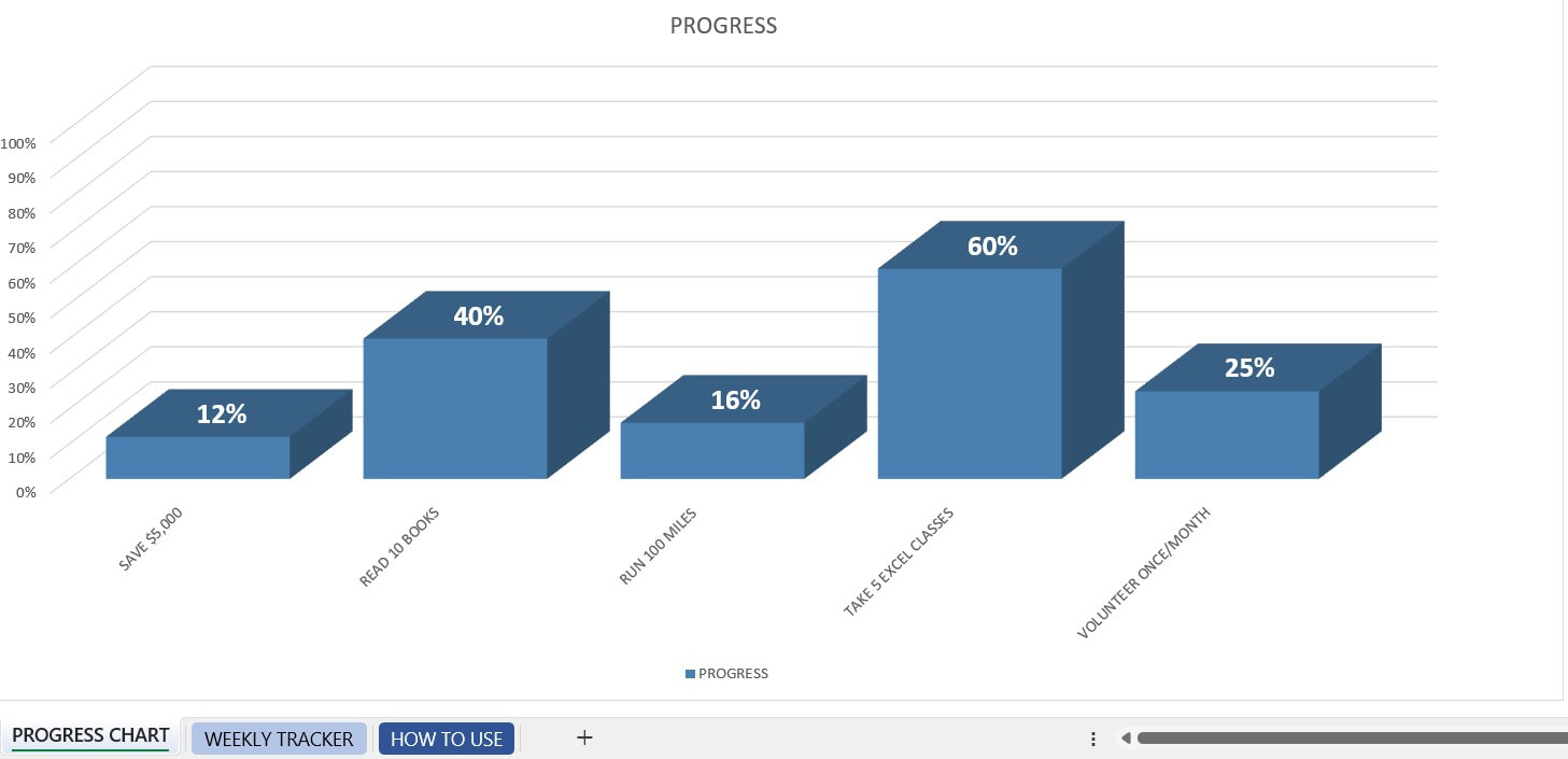 Data bars are super easy to set up and don’t require any chart building skills! 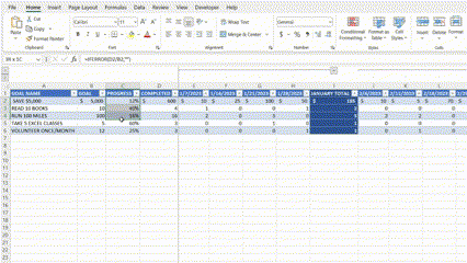
This is a drop down menu, so you will hover over Data Bars and then select the color that works best for you. 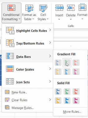 Once you select your data bars, you’ll see them fill into each of your selected cells depending on the value in each cell. 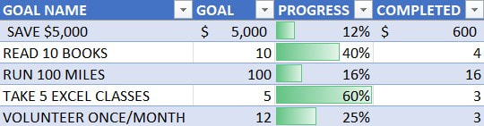 You’ll notice that your 60% is filling the entire cell and that is because it is the largest value and it has the other bars set in comparison to the 60%. To change this to be a true tracker to 100%, you need to edit your conditional formatting. Go back up to Home and then Conditional Formatting. This time, instead of selecting Data Bars, you’re going to go down to the bottom of the drop down and select Manage Rules. Once you open the rules manager, you will see all of the conditional formatting rules you have set up. You should select the one for data bars and then click Edit Rule. You will see you have a section that says Minimum and Maximum with a Type and Value. This is likely showing “Automatic” for Minimum and Maximum which is why the 60% is filling the entire cell with the bar because it’s reading the 60% as your maximum. You will want to change this to either number with your values set from 0 to 1 or you can select percentage for your type and 0 to 100 in your values. This will now show a 0% as no bar and 100% as a full bar.  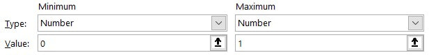 This will now show a more appropriate 60% bar. 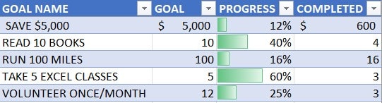 There are a lot of great Conditional Formats that you can include in your Excel documents to make the data easier to read. Play around with it and let me know if you’d like to see what else we can do with Conditional Formatting!
0 Comments
I’ve covered the amazing trick of copying the sum, average, or count of your selected cells by clicking your subtotal amount at the bottom of your screen. If you missed that, it’s a super short read here. This is a great tip, but what if you need something besides the sum, average, or count? We also have access to numerical count, minimum value, and maximum value and we have the option to turn off any of the default options. If you only want to have sum available, you can choose to remove the other options. 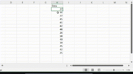 To add or remove the other options, you just right click on the lower border of your Excel (the status bar) to open the Customize Status Bar menu. You will see the options of sum, average, and count already checked by default. You can click those to uncheck them or you can check the others to add them to your lower bar.
This is a super easy way to make Excel customized for what you need to access most to make you faster and more efficient! Drop-down menus or drop-down lists are an easy way to elevate your Excel document. They make forms look professional and make it easy for the user to make a selection that is uniform in phrasing and formatting. This can be extremely helpful if you use the drop-down selection for a lookup to populate other data. We’ll cover how to set up a single drop-down menu, a dependent drop-down menu where the first selection triggers the options for the second menu, and a drop-down that triggers a lookup to pull in a result based on the selection. 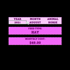 Basic Drop-Down MenuTo set up a basic drop-down menu, you need to create a list of your menu options. For my example, I have a list of animals that I would like to be the options in my drop-down. 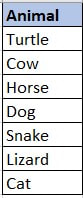 Next, we need to decide where the drop-down will live. I have created an Animal header and want the drop-down to live in the cell under that in A2. First, I will click into A2, then go to Data>Data Tools>Data Validation. If you are on a smaller screen, it may just be a small icon next to Text to Columns. 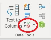 When you click the icon, you will open the Data Validation popup. You will use the drop-down menu under Allow to select List. This will change the next options to now have a Source field. You can either type in the location of your list, or you can click and select the cells that contain your list. Since my list of Animals is in K2 through K8, I have selected those cells. It automatically locked my cells with the “$” which is great because if I were to drag my data validation down so I have multiple cells with the drop-down, it will continue to pull the same list. 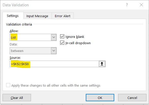 You can also name the range that contains your list and use that name in your source. Click this link to learn how to name ranges and manage them. 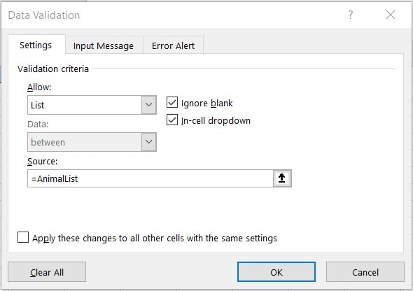 You’ll see you now have a little arrow button when you click into A2. 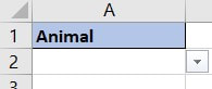 If you click that button, you will see your list appear and you can select off of the options from your list. 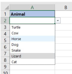 When you select from your list, your selection will display in the cell. 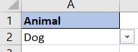 If you want to clear your selection, you can select the cell and hit delete. This will still keep your drop-down list active, but just clear your selection. To remove your drop-down completely, select the cell, go back to Data Validation as if you were going to set it up but instead click Clear All and then OK. 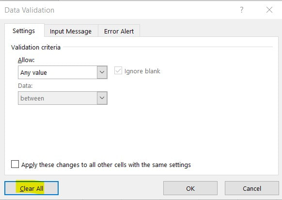 Dependent Drop-DownsIf we have multiple lists that we want to have shown in a drop-down based on what the first selection is, we can create a dependent drop-down. For our example, you will first select an animal class (mammal or reptile) and then the second list will give you the animals that belong to that class. For this, we will need to name each of our lists with the same name as the label that exists in the first drop-down. For example, if in the first list we have Mammal and Reptile, then we need to name our list of mammals as “Mammal” so when Mammal is selected, Excel is able to match the range. We will start with the first drop-down which will follow the same set up as above: Data>Data Tools>Data Validation and select List under Allow and your list range or range name under Source. Next, we need to add our drop-down for the dependent cell. We will start with the same steps Data>Data Tools>Data Validation and select List under Allow. For the Source, instead of selecting a range of cells or your named range, you are going to use the formula =INDIRECT(A2) where A2 is the cell that your primary drop-down is.  This is looking in A2 for the range name and then pulls the list for that range. 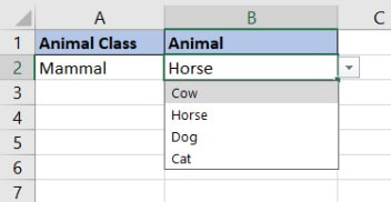 Using a Drop-Down in a DashboardIn creating dashboards, a drop-down might be a useful tool to help your user filter right to the data that they’re interested in without having to look through all of the information. For my example, I have a data set with the Feed Cost for each of my individual animals for the past two years by month. I also have the animal type, animal’s name, and the feed type. I want to create a dashboard where I can select which month, year, and animal to see what the feed type is and what the feed cost was that month. Since my data set is so long, I don’t want to create my drop-down list directly from the data since I will have so many duplicate labels. I started by creating a separate section with the headers of the drop-downs that I wanted to include and then used =UNIQUE(M3:M74) to pull a list of unique values from my data for Year. I repeated this for Month, Animal, and Feed Type. 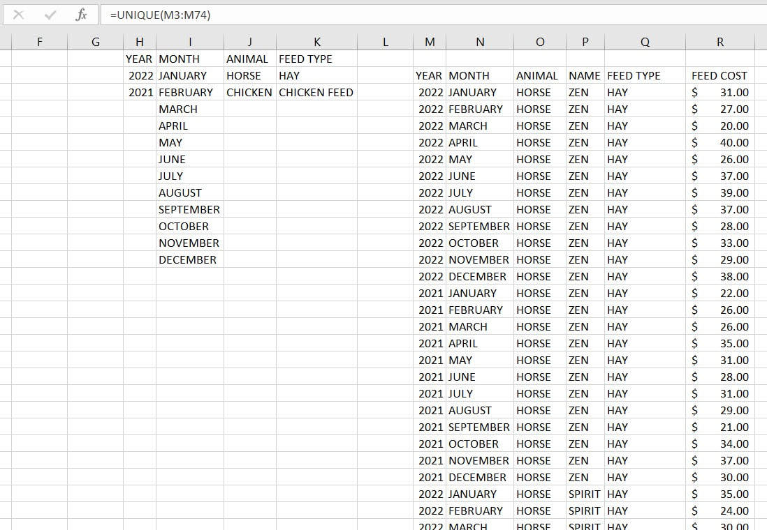 Where I want my dashboard to be built, I set up my drop-ship for each of these columns. 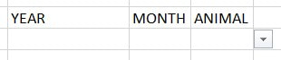 I want my dashboard to display the feed type and the feed cost, so first I will use the dropdown option for Animal to do a XLOOKUP for the feed type. If you need a refresher on XLOOKUP, check out my guide. 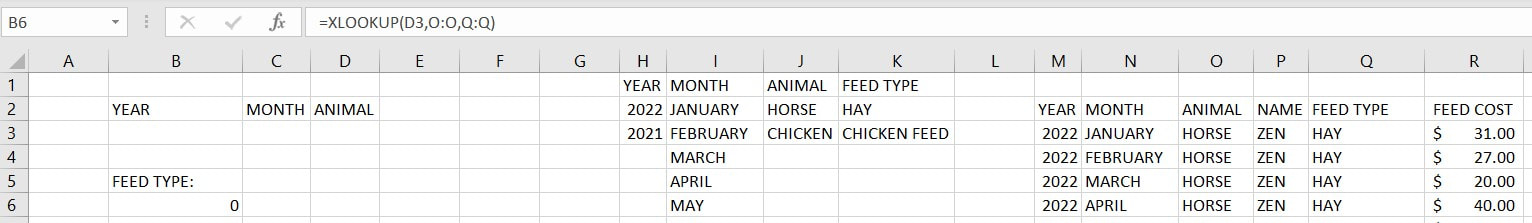 When I select an animal, the feed type now populates. Since each of my animal types only eats one type of food, this works perfectly. If I had changed my food type at a certain point in time, I would also include the year and month to pull in the feed type in that year and month. 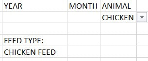 Next, I want to show the total feed cost when a year, month, and animal is selected. Since I have multiple horses, I want this to be a sum instead of a lookup so I can see my total cost for all of my horses. For this, I will use =SUMIFS since I have multiple conditions with year, month, and animal. 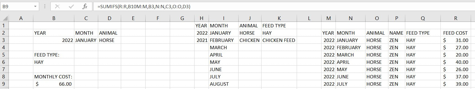 Now, if I change any of my drop-downs, my results will automatically update. 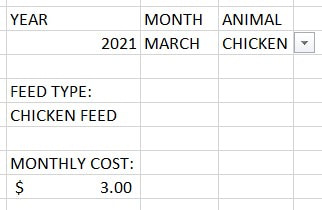 This is exactly what I wanted, but it’s just not very pretty. With some formatting, we can get this to look a little nicer. 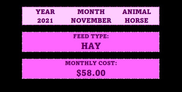 Now we have a really nice looking dashboard that we can adjust and include in our presentations. I'd love to hear what you plan on using drop-down menus for! Let me know in the comments below.
Did you know that you can name specific cells in your Excel workbook? Let’s say you have a list of animals in A2:A10, you can name that list “Animals”. Sounds cool, but what would you need that for? Well, if you need to reference these cells in formulas or functions and you have multiple ranges named, you can just put your name right in the formula/function instead of having to type the range or going and selecting the range. For example, you can use this for a lookup like =XLOOKUP(F1,Animals,Price) where Animals is your list of animals in A2:A10 and Price is your list of prices in B2:B10. F1 is the animal you want to go look for. If you want to learn more about XLOOKUPs, check out my guide here: https://www.excelbyashley.com/guides/xlookup. A benefit to using named ranges is you don’t have to lock your reference cells. If you had used A2:A10 in your XLOOKUP and then dragged your formula down a list of different animals, you would have to lock your reference cells to be $A$2:$A$10 otherwise it would shift to A3:A11, A4:A12, etc. as you drag it down your list. Learn more about locking reference cells here: https://www.excelbyashley.com/guides/how-to-lock-a-reference-cell-in-an-excel-formula. You can also use this in a formula like =SUMIFS(Price,Animals,"T*") where you are getting the sum of Price for anything in Animals that begins with a T. Dependent drop-down reports also rely on your ranges being named which will be covered in a later lesson. Let’s go over how to name a range. You have a few methods available. The first way is to select the cells that you want included in your named range and then click into the box in the upper left corner next to your formula bar. Typically this box shows you the cell name of what you have selected, like C5. Once you click into this box, you can type your range name and then hit enter to save. The rules are that your name needs to be one string of text without spaces and it cannot be a cell name like AA3. 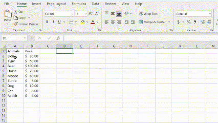 Once you have named your range, you can see your range name in the drop-down from that box where you set the name. You can also select the same range and you will see your range name in the box. 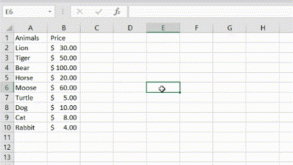 The second way to name a range is to use your headers to your advantage with the “Create from Selection” tool. With this one, you’ll select the entire range including your header. You’ll go to Formulas in your ribbon and then click “Create from Selection.” You will get a popup asking where to pull the name from: Top Row, Left Column, Bottom Row, or Right Column. Since I have my header in the top row, I leave it on default to Top Row. This will take my top row from my selection and use that as the name of the range with the actual range of data starting in row 2. 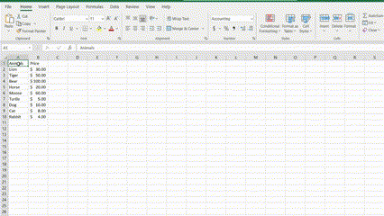 The third way you can name a range is through the Name Manager in the Formulas tab of your ribbon. Start by opening the Name Manager. Here, you will see any ranges that already exist in your workbook. This is a great tool because it allows you to edit or delete an existing range. You can also create a new range by clicking New. If you select your cells before opening the Name Manager, it helps you by detecting the possible Name and Range that you’d like to create. If you don’t have a range selected, you may select a range from the pop up or type one in. You can also type any name that you’d like along with any comments. The comments will show up in your Name Manager and may be helpful if you are sharing your document. 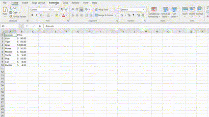 Define Name and Use in Formula may also be helpful to you in creating your named ranges or using them in your report. Play around with it, find what works best for you, and let me know what you are using named ranges for!
Sometimes we are not in control of the data that is provided to us or the format we are able to export in and we end up with an Excel sheet that shows data lines in more of an outline format. This will look like an outline that flows in a hierarchy where the first column has the header that the next column rolls up to and then the next column shows the parts of the second column labels. You may need to fill in your blank cells so each row has complete data and you can sort, filter, apply IF formulas, and create PivotTables. 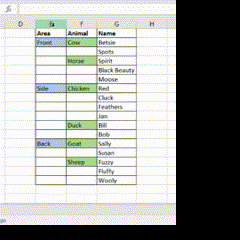 There is a pretty simple fix for this that you can do in under 30 seconds, you just have to know how! 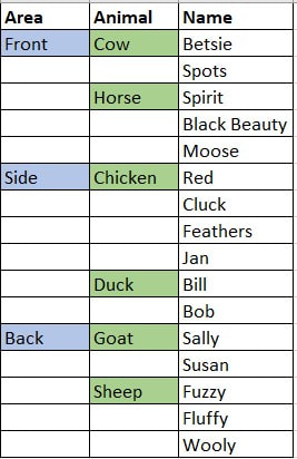 Start by highlighting your dataset. Next, go to Find & Select in the Editing section of your Home ribbon. You can also use the shortcut CTRL + G. 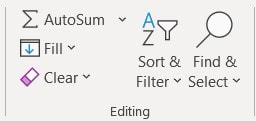 Select Go To Special or use the shortcut ALT + S to open the Go To Special popup. 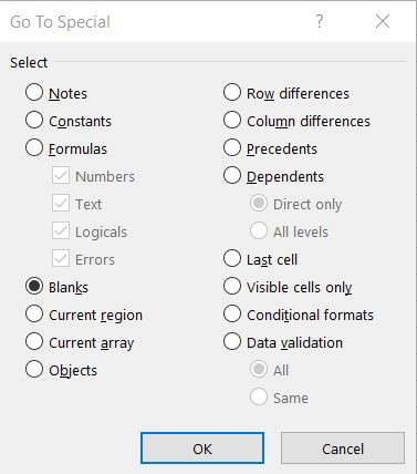 Then select Blanks or use the shortcut ALT + K. Hit OK or ENTER. This will result in only having the blank cells selected. Next, you need to enter a formula to tell Excel what to do to those blank cells. Type “=”, then hit the up arrow, then hit CONTROL + ENTER at the same time. This is starting a formula by typing = then it’s selecting the cell above what you have selected. This defaults to your first blank cell so it will select B2 if your first blank is in B3. This is writing the formula =B2 meaning that the cell you’re in will now display the same text as the cell above it. By clicking CTRL + ENTER it applies that formula to everything that is selected so each blank cell now displays the text of the cell above it. You can do the same action if you need it to match the cell to the left or right instead by just selecting a different arrow key. 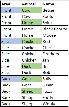 You can see we have filled in all of our blanks to now match the cell above them. You will need to then copy your cells and paste as values to remove the live formulas if you wish to sort these. Reach out if you get stuck or let me know how it worked for you in the comments!
I love a good theme, so as we enter this new year, let’s go over the little known function that calculates how much time is between two dates. This can be used to find how many days it has been since a date (past due), how many days it will be until a specific date (days until due), or days between two dates like how far apart two siblings are. This function also allows us to measure time in different units such as days, months, or years! 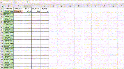 The formula is simple: =DATEDIF(start date, end date, “units”)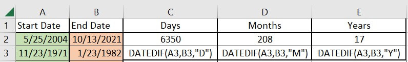 You can enter the start and end dates as references to another cell, you can type in a date, or you can use the Today() function to compare to today. If we want to type in the date for either the start or end date, we need to put it in quotation marks. 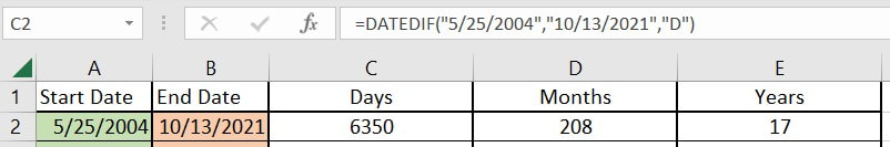 If we wanted to use the Today() function as our end date it would look like this: 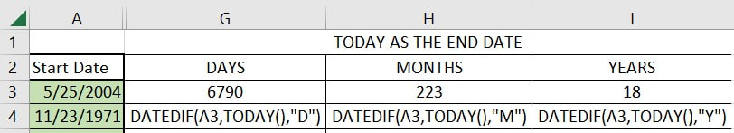 The units that you specify should also always be in quotation marks: “D”, “M”, “Y”. This could be helpful if you need to show how many months there are until a due date on an invoice. 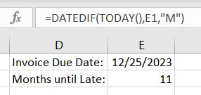 Note that the Year and Month units will show the number of complete years/months until that date. If today is 12/27/22 and I’m doing a DatedIf to 12/25/2023, there is less than 1 complete year, so my result will be 0. 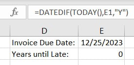 If you have any issues or questions, please reach out by sending an email!
If you have ever selected a few cells, looked at the bottom of your Excel screen to see the subtotal, and repeated the numbers really fast to yourself so you could type that subtotal somewhere else before you forgot, this is the lesson for you!! Maybe you even keep some scrap paper to jot down that sum so you can go put it in your recap email. Or maybe you create a quick =SUM cell off to the side so you can copy that into your commentary and then have to remember to clear that cell later. Well, there is a better way. I’m not sure why this isn’t common knowledge, but once I learned this, it was a GAME. CHANGER. It’s so simple it makes me mad that nobody told me about this, so here I am, spreading the word!  You just click on the sum at the bottom of your Excel screen and it automatically copies it. This allows you to paste the sum, count, or average subtotal into another cell, document, presentation, or e-mail.
You will never repeat your subtotal in your head while you change screens again. I hope this makes you just a little more efficient today. Let me know in the comments if you already knew this one or if it just blew your mind as much as it blew mine! Happy New Year! New Year Resolutions sound so negative to me, like we’re focusing on what we want to give up instead of what we want to accomplish. I looked up the origin of “resolution” and found “from resolvere ‘loosen, release’ (see resolve).” I don’t want my year to start with a focus on just what I’m giving up or releasing, but instead what I’m gaining and accomplishing. As we all reflect on this last year and look forward to the next and all the possibilities it may bring, I found myself creating lists of all the things I want for myself in the next year. Since my birthday is right before New Year’s, not only is the calendar changing, but I’m entering a new age. In this next year of my life, I have some big goals and need a way to track them all. To keep me motivated throughout the entire year, I want to see that I’m progressing toward accomplishing my goals so, of course, I turned to Excel. Excel offers me a tool that can calculate my progression plus it can give me a graph as a visual so I can see just how much I’ve done! I’ve attached my goal tracker here to encourage you to make some goals of your own for this new year. I think setting this up in a weekly format will keep us accountable in bite sized pieces. Just set a reminder each week to log what you’ve done and you’ll see your graph grow as you approach 100% on each of your goals. 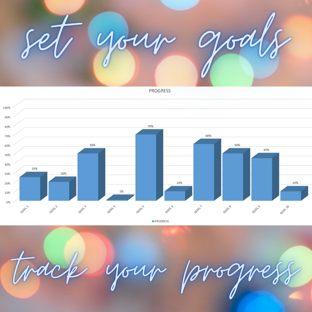 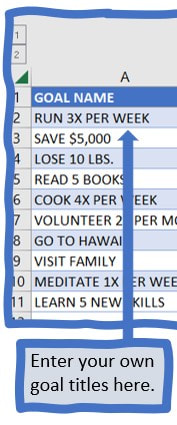  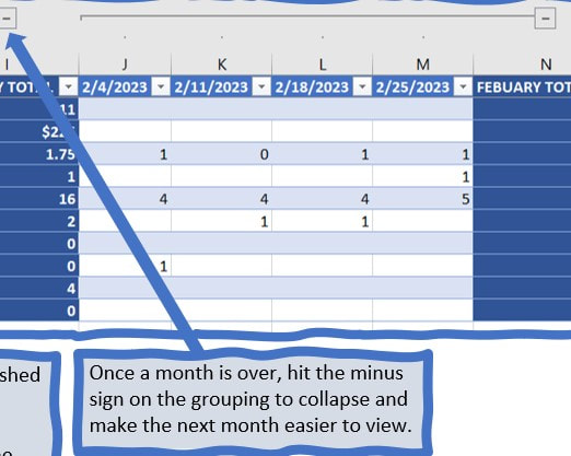 I hope this is easy for Excel users of all levels to implement. I wanted to keep it simple and straightforward. This one isn’t about improving Excel skills, but just taking a few moments for yourself to improve your life. I hope you enjoy. Happy New Year.
Excel may not be where you think to turn for a creative project, but there are actually some fun tools that you can use to make your Excel document a little more artistic and fun! It is almost Valentine’s Day, so I will show you how to make an Excel Valentine to send to all your favorite Excel friends.  We will start with a fresh Excel document, but these steps can be applied in an existing sheet alongside your data if you’d like. First, go to View and uncheck the Gridlines box in the Show section. This will remove the gray gridlines so our sheet is a blank space instead of showing all the cells.  Next, we will fill the cells with the background color of your choice. You will click the arrow in the upper lefthand corner between A and 1 to select the entire sheet. You will select a color to fill your background from the paint bucket in the Font section on the Home tab of the ribbon. I’m choosing a gray background for my Valentine. 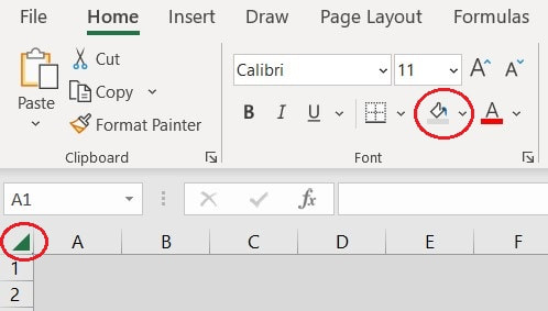 Next, we will insert the heart shape on our sheet. Go to the Insert tab on the ribbon and select the Shapes drop down menu. For this project, we will select the Heart shape. 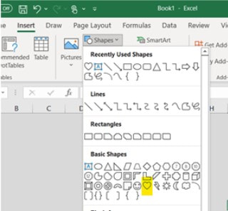 Once you select the shape you want, your cursor will change to a plus sign. You can click anywhere (I usually start in the upper left corner of where I want my shape to start) and then drag down to the shape and size that you want. When you release your mouse, the shape will be placed. If you click on it, you can adjust the placement and sizing. 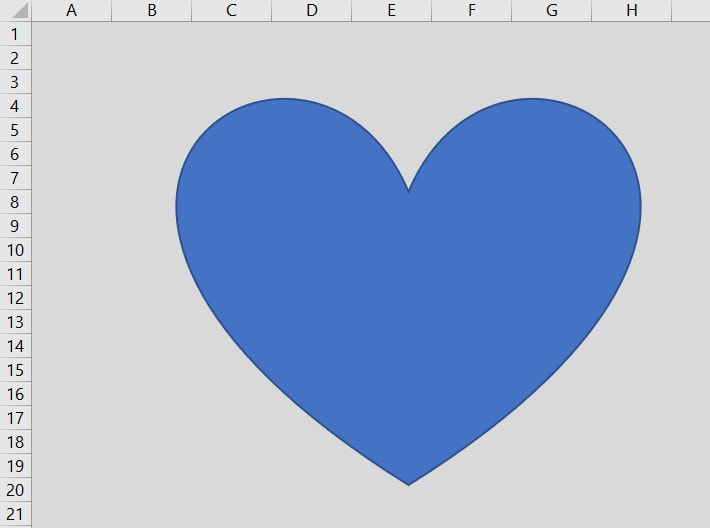 We will use this first heart to be our background heart which will act as the box. We first need to change the fill to a dark red and the outline to black. You can do both of those in the Shape Format tab of your ribbon which appears when you click on your shape. From the dropdown of the Shape Fill we chose our red and the Shape Outline we chose black.  Next, we need to duplicate our heart for the chocolate part. You can copy your existing heart by right clicking on the heart or using control C and then paste using right click or Control V, or you can go back through the steps we just did. We want to resize the second heart to fit inside the first one so it looks like the inside part of a heart box. When you click on the heart, you will see there are dots in the corners. When you click and hold those, you can adjust the size and shape of the heart. You can also right click on the heart and select Edit Points to adjust the parts of the heart. This is the hardest part of the project, but you just have to play around with it until you’re happy with how the hearts align.  Now we get to be creative! Select the smaller heart and go back to your Shape Fill dropdown. At the bottom of the dropdown menu, you will see an option for Picture. 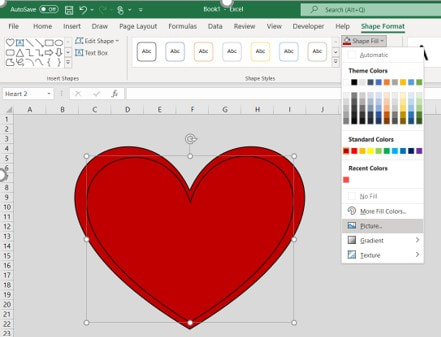 Once you click Pictures, you can select where to get the Picture. If you would like to insert a picture of you and your work bestie, you can select From a File. You can also browse the Stock Images or Icons that Excel provides, or you can look for pictures online. I’m going to select Online Pictures. 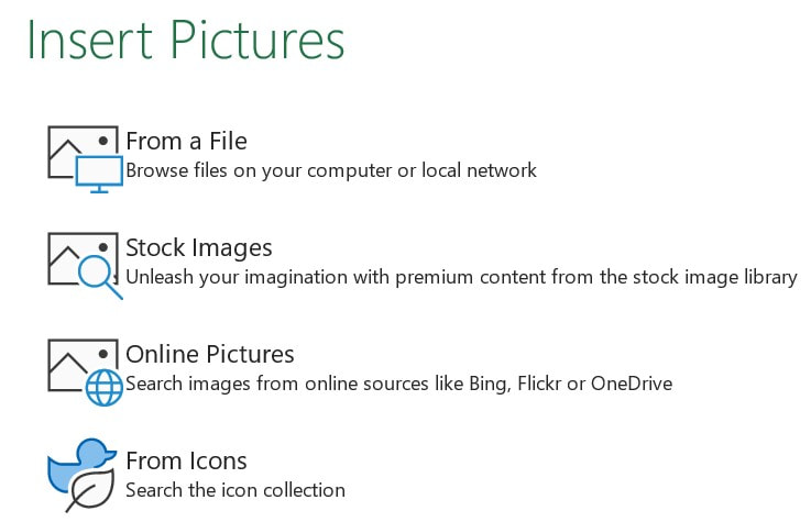 You will get a popup with a search bar. I am going to search for “Chocolates”. 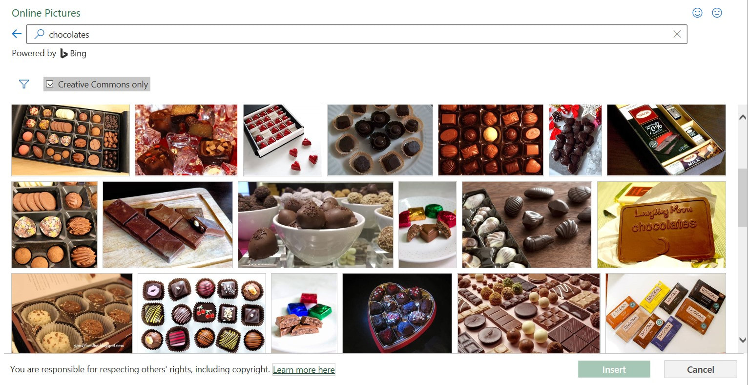 You can scroll through the results and find the one that best fits what you need and then click Insert. It may take a few search options to get the perfect result for your project. Once you click Insert, the image will fill into the shape you had selected.  This is really starting to take shape, but it’s still pretty flat. To add some depth, we will play with the shape effects. Let’s start with the bigger heart. Go back to your Shape Format tab in the ribbon and under the Shape Fill and Shape Outline that we already used, there is Shape Effects where you can add shadows, glow, 3D and more. I’m going to use one of the Bevel settings to add depth. I selected Bevel Angle. You can see when I hover on it, it gives me a preview of what the shape will look like with this applied. 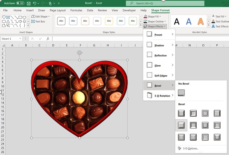 I also want to add some 3D effects so I will apply Oblique. 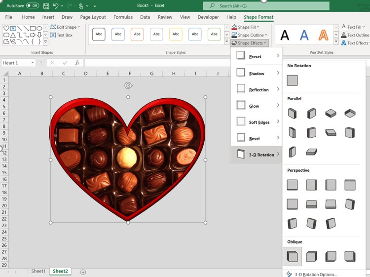 Next, I want a shadow, so I will select Shadow>Perspective from the same Shape Effects menu. 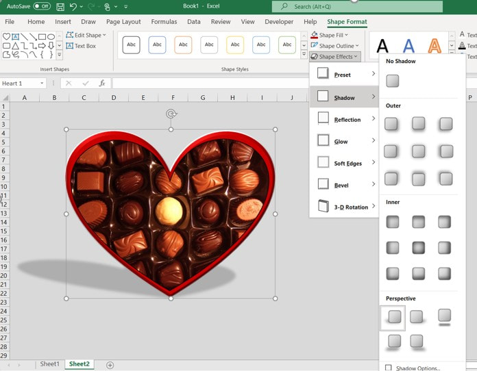 I will also apply a shadow on the chocolate heart by clicking on the smaller heart shape, going to Shadow and selecting Inner Center. 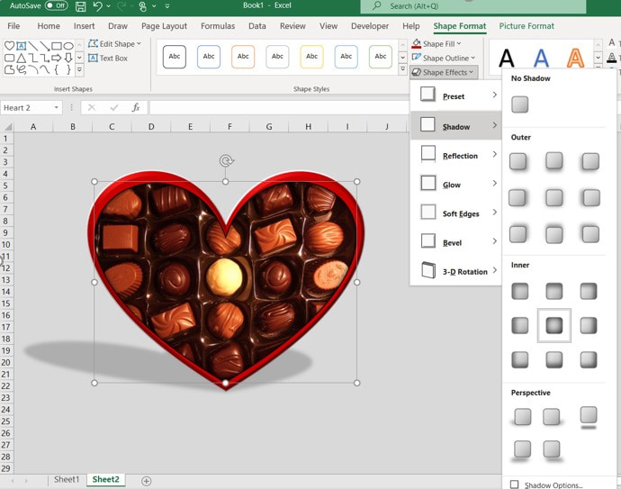 Next, we can add our custom message! Go to Insert>Text>WordArt which is located on the very right side of the Insert ribbon. 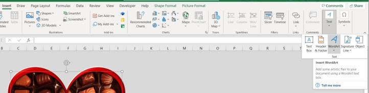 Once you select WordArt, you will have a drop down menu of some common options. You can choose the one that most closely looks like what you’d like the final result to be, but we will be making a lot of changes. Here’s what mine looks like to start:  With your WordArt still highlighted, you can start typing the word or phrase you’d like your WordArt to say. I put “Happy Valentine’s Day.” If you right click on the text box, you will see a menu of options including some quick formatting adjustments. 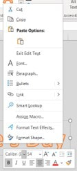 To start, I will make the text a few sizes smaller and change the text color to white. I will also change the font type to Brush Script MT. Similar to the Shape Fill and Shape Outline under the Shape Format tab of the ribbon, there are Text Fill, Outline, and Effects. We will apply a black outline.  I will relocate this WordArt and center over my chocolate heart by clicking the text box and dragging. Then I can adjust the size of the text box to get the words aligned how I’d like. If I narrow the box, the text will wrap on three separate rows.  I want this text to stand out from the chocolates a little more, so I will apply a glow effect in red. I use the Text Effects dropdown just like I did with the Shape Effects. I select Glow this time and go down to more colors to select bright red. 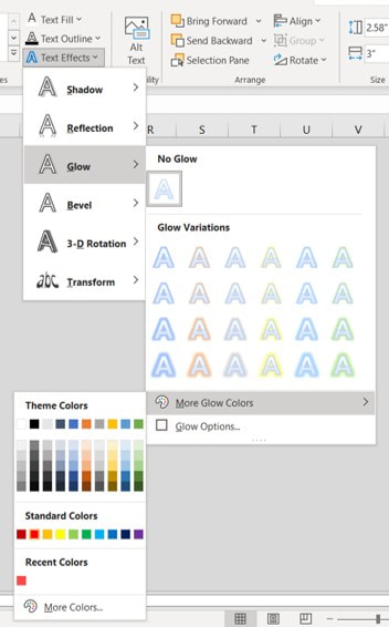 The text now stands out from the dark background.  Now I’d like to angle the text. If I click on the text box, I get the dots in the corner to resize and I also get a circle arrow in the top center. This is to rotate the text box. I will click and drag it into the position that I’d like. 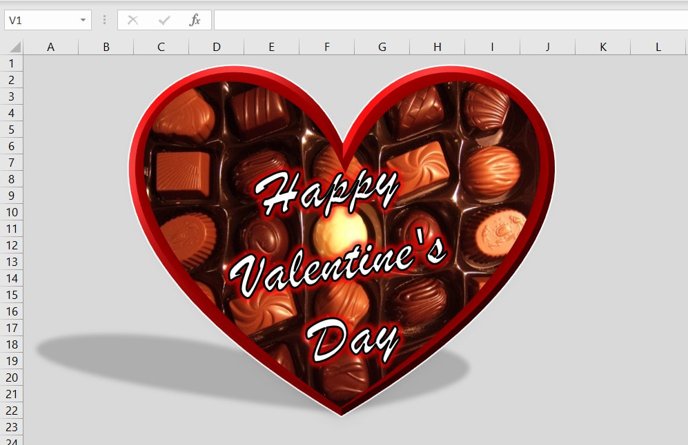 This is ready to send! You can play around with these settings and do all kinds of fun things. Maybe you fill a shape with a company logo or picture. This could be used to make your spreadsheets more interesting, to spice up your invoices, or to make a funny surprise for your coworker! Let me know in the comments how you’ve used Shapes or WordArt in your Excel documents. If you have any issues or questions, please reach out by sending an email!
|
|||||||||||||

